原文: INVERSE KINEMATICS AND GEOMETRIC CONSTRAINTS FOR ARTICULATED FIGURE MANIPULATION

http://graphics.ucsd.edu/courses/cse169_w04/welman.pdf

译者: crazii

http://www.cnblogs.com/crazii/p/4662199.html

[译者: 根据个人需要, 只仔细阅读了部分内容, 所以只翻译 基本概念(3.1)和 CCD相关(4.2, 4.3) 的部分. 后面如果有空的话, 可能选择翻译一下第5章 约束(Incorporating Constraints)的问题.p.s.本人渣数学, 很多术语可能翻译不准确. 还有一些句子是意译.为什么只翻译CCD, 而不翻译雅克比转置法? 因为首先阅读了4.3章, 两者的比较, 发现CCD实现更简单, 收敛速度更快(效率高), 没有奇点等优点, 所以就选定了CCD.]

第三章 反向动力学 (逆向運動學) - Inverse Kinematics (IK)

反向运动学的问题, 在机器人技术的文献中已经得到了广泛研究, 目前仍然是该技术领域内最好的信息源. 在这一章里我们会正式的提出这个问题, 并回顾最常用的IK解决方法, 并描述在此之前这些方法在计算机图形学中的一些用例.

The inverse kinematic problem has been studied extensively in the robotics literature, which remains the best source of information on the subject. In this chapter we formally state the problem and review the most common approaches to solving it. Previous applications of these approaches to computer graphics are also described.

3.1 反向动力学问题 - The Inverse Kinematic Problem

第2.1.2章节(骨骼建模)中, 描述了一个骨架可以这样建模: 由一些被关节连接的刚体, 按一定的层次集合而成. 我们把骨骼中的由各段组成的一个运动链称作操纵器(manipulator), 并假定这个运动链中, 连接两段之间的关节是只能绕一个轴旋动的旋转关节. 操纵器链条的一端, 即基座(base), 是固定的无法移动; 链条的末梢一端可以自由移动. 末端效应器(end-effector, 下称末端器)位于最末端关节的坐标系(coordinate frame)中; 末端器的坐标是该坐标系中的一个点, 末端器的朝向(旋转)与该坐标系的朝向一致.

Section 2.1.2 showed that a skeleton can be modelled as a hierarchical collection of rigid objects connected by joints. We will refer to a kinematic chain of segments within a skeleton as a manipulator, and will assume that the joints connecting segments within this chain are revolute joints rotating about a single axis. One end of the manipulator, the base, is fixed and cannot move; the distal end of the chain is free to move. The end effector is embedded in the coordinate frame of the most distal joint in the chain; the end-effector position is a point within this frame and the end-effector orientation refers to the orientation of the frame itself.

对于这个运动链中的每一个关节点, 用一个关节变量来表示这个节点处的两个相邻坐标系的空间变换M, 在每个旋转关节i处的变换 Mi 由位移和旋转构成, 这两个量是相对于父节点坐标系的相对值, 即

Mi = T(xi, yi, zi) R(θi)　　(3.1)

其中T(xi, yi, zi) 是从父关节节点i-1到当前节点i的位移矩阵, R(θi)是绕着关节i的旋转轴旋转了θi的旋转矩阵.

At each joint in the chain a joint variable determines a transformation M between the two adjacent coordinate frames sharing the joint. The transformation Mi at a rotation joint i is a concatenation of a translation and a rotation, both of which are relative to the coordinate frame of joint is parent. That is,

Mi = T(xi, yi, zi) R(θi)　　(3.1)where T(xi, yi, zi) is the matrix that translates by the offset of joint i from its parent joint i, and R(θi) is the matrix that rotates by θi about joint is rotation axis

这个运动链中, 任意两个关节的坐标系i和j的关系,可以由从i遍历到j时,遇到的所有节点的变换相乘求得:

Mij = MiMi+1...Mj-1Mj　　(3.2)

所以与基座坐标系相关的末端器的位置和朝向, 可以简单的由每个节点的变换相乘求得. [译注: 若基点处的变换为M0, 末端器的变换为Mn, 则由上式可得 M0n=M0M1...Mn-1Mn 即所有节点局部变换的乘积.]

The relationship between any two coordinate systems i and j in the chain is found by concate nating the transformations at the joints encountered during a traversal from joint i to joint j:

Mij = MiMi+1...Mj-1Mj　　(3.2)

So the position and orientation of the end-effector with respect to the base frame is found by simply concatenating the transformations at each joint in the manipulator.

如果一个链中的的已知节点变量组成的向量为q [译注: q = (M0, M1, ... Mn)], 那么前向运动学(forward kinematic)中, 计算末端器的坐标和旋转的向量x的问题 [译注: x = (T, R)], 是一个简单的矩阵乘法的问题, 格式如下:

x = f(q)　　(3.3)

然而如果目标是将末端器放置在给定的位置和朝向 x, 那么计算合适的节点变换向量q来达到目标的问题, 需要解决(3.3)的逆, 

q = f-1(x)　　(3.4)

解决这个逆向动力学的问题就没有那么简单了. 函数f是非线性的, 而且如果存在一个x到q的方程(3.3)的唯一的一个解, 那么逆向的q到x映射(3.4)未必只有一个 - 对于给定的x, 可能有多个q的解存在 [译注: 直观的表现是抵达同一个点可能有不同弯曲的方式, 比如""形,两种]. 解决这个问题的最直接的方式可能是求出方程(3.4)的解析解(closed-form solution). 但是解析解使的场合非常有限, 只适用于那些具有特定特点的操纵器[译注: 比如旋转的角度/自由度受限, 比如, 所有节点只有1个自由度DOF], 甚至这种情况仍然需要解非线性方程[Pau81]. 对于任意的一个操纵器, 通用的分析解法是不存在的; 相反, 问题需要通过非线性方程的解法中的数学方法. 最常用的解法是基于矩阵求逆或者优化技术(optimization techniques).

Given a vector q of known joint variables, then, the forward kinematic problem of computing the position and orientation vector x of the end-effector, is a simple matter of matrix concatenation, and has the form

x = f(q)　　(3.3)

But if the goal is to place the end-effector at a specied position and orientation x, then determining the appropriate joint variable vector q to achieve the goal requires a solution to the inverse of(3.3)

q = f-1(x)　　(3.4)

Solving this inverse kinematic problem is not so simple. The function f is nonlinear and while there is a unique mapping from q to x in equation(3.3), the same cannot be said for the inverse mapping of(3.4) - there may be many qs for a particular x. The most direct approach for solving the problem would be to obtain a closed-form solution to (3.4). But closed-form solutions can only be derived for a restricted set of manipulators with specfic characteristics, and even these result in a set of nonlinear equations to be solved[Pau81]. A general analytic solution for arbitrary manipulators does not exist; instead the problem must be solved with numerical methods for solving systems of nonlinear equations. The most common solution methods are based on either matrix inversion or optimization techniques.

第四章 直接操纵的有效算法 Efficient Algorithms for Direct Manipulation

4.1 一个简化的动态模型 A Simplied Dynamic Model

4.1.1 雅可比转置法 The Jacobian Transpose Method

[以上暂不翻译...]

4.2 一个补充的启发式解法 - A Complementary Heuristic Approach

上述的基于力(force-based)方法, 对于互交式操纵来说有着比较吸引人的一些特点.然而有些情况下,这种方法的表现并不能尽如人意. 图4.2说明了其中的一种情况. 左边是一个奇异构形(singular configuration)的操纵器, 黑点表示的是末端的新的期望目标位置. 右边的形态显示了对该IK问题的一个合理的解, 可能也反映了用户所期望的, 将末端向内拖至目标的结果. 然而当用户尝试将末端向内拖动时, 在末端施加的力直接指向奇异方向(singular direction); 这个力会被抵消而毫无效果, 而末端并不会移动. 考虑到雅可比转置法作的物理类推, 这个结果是合理的, 但实际上它可能并不符合用户的期望.

The force-based approach of the preceding method has some appealing characteristics for interactive manipulation. There are some cases, however, for which the method does not perform well. Figure 4.2 illustrates one such case. On the left is a manipulator in a singular conguration with a new desired position for the tip shown as a black dot. The conguration on the right shows a reasonable solution to this inverse kinematic problem, and probably reflects what a user expects to get by dragging the tip in towards the goal. However as the user attempts to drag the tip inwards the applied force exerted on the tip points straight down the singular direction it is in effect cancelled out and the tip will not move. This behaviour is reasonable given the physical analogy of the Jacobian transpose method, but may not really match the users expectation.

图4.2: 一个雅可比转置法不能很好处理的情况. 左图向内拉动操纵器的末端并不能生成如右图所示的期望结果.

这里展示一个替代的IK算法, 适合于互交定位, 而且对于图4.2的情况, 能够提供合理的结果. 它基于一种启发式方法, 这种方法的提出, 是用来为一个标准的基于最小化的算法快速地找到一个初始可行解(initial feasible solution) [WC91]. 然而它可以独立作为一个IK定位的工具, 像雅可比转置法一样, 这种方法既简单又有效, 而且可以解决带有奇点的问题. 然而它的行为与前面演示的算法差别比较大, 这里建议将它作为雅可比转置法的一个补充, 而不是替代.

An alternative inverse kinematic algorithm is presented here, suitable for interactive positioning and capable of providing reasonable behaviour in cases such as that in Figure 4.2. It is based on a heuristic method which has been proposed to quickly find an initial feasible solution for a standard minimization based algorithm[WC91]. However it can stand on its own as an inverse kinematic positioning tool. Like the Jacobian transpose method the technique is efficient, simple, and immune to problems with singularities. However its behaviour is quite different from that exhibited by the previous algorithm, and it is suggested here as a complement to, rather than a replacement for, the Jacobian transpose method.

4.2.1 循环坐标下降法  The Cyclic Coordinate Descent Method

循环坐标下降法是一个迭代的启发式搜索技术, 它尝试通过每次修正单个关节, 将位置和朝向的误差最小化. 每次迭代都需要对操纵器进行一次从末端关节到基座的遍历. 为了将目标函数最小化, 每个关节变量qi会按顺序被修改. 单个关节上的最小化问题是足够简单的, 可以构造出一个分析解, 所以每次迭代都很快.

The cycliccoordinate descent (CCD) method is an iterative heuristic search technique which attempts to minimize position and orientation errors by varying one joint variable at a time. Eachiteration involves a single traversal of the manipulator from the most distal link inward towards the manipulator base. Each joint variable qi is modied in turn to minimize an objective function. The minimization problem at each joint is simple enough that an analytic solution can be formulated, so each iteration can be performed quickly.

由于对于每个关节都得到一个解, 末端器的坐标和朝向就可以立即更新以反映出这些变化. 因此在当前迭代中, 任何一个关节上的最小化问题, 都包含了对末端那些节点的修改, 对它们产生影响. 这与之前描述的方法不同, 之前的方法实际上是同一时刻确定每个节点的变化2 [2:原作者注: 虽然每个节点的变化是按顺序计算的, 但是父节点不对子节点产生影响, 迭代过程中操纵器的状态不变].

As a solution is obtained at each joint the end-effector position and orientation are updated immediately to reect the change. Thus the minimization problem to be solved at any particular joint incorporates the changes made to more distal joints during the current iteration. This differs from the previously described method, which in eect determines the changes to each joint simultaneously2 (2: ie although the changes are computed sequentially, the state of the manipulator remains constant during the iteration).

[译注: CCD是将末端效应器与目标的距离作为启发函数, 通过每次迭代时, 通过调整旋转, 不断逼近目标, 将与目标的旋转和位移误差最小化, 最后达到目标. 由于每次迭代是从末端开始到基座, 靠近基座的关节会对靠近末端的节点产生影响, 在处理每个关节点之前, 其子节点的误差已经最小化. 下面是对每次个关节上问题的分析, 实际使用中可以根据原理, 作出各种应用和工程的算法.]

假定当前的末端器坐标是

Pc = (xc, yc, zc)

而末端器的朝向, 是由旋转矩阵Oc的三个正交向量确定

Oc = [ u1c, u2c, u3c]T [译注: 原文中是列向量, 这里不好表示, 故写作行转置]

要想使末端器离目标位置Pd和目标朝向Od尽可能的接近, 需要找到一个关节向量q, 使得下面的误差最小化:

E(q) = Ep(q) + Eo(q)　　　　　　(4.13)

它是位置误差

Ep(q) = ||(Pd - Pc)||2　　　　　　(4.14)

和朝向误差

Eo(q) = ∑j=13 ((ujd·ujc) - 1)2　　(4.15)

两者之和.

这个方法在计算时每次只考虑一个节点, 从末梢开始计算, 直到基座. 计算到下个节点i-1之前, 每个节点变量qi会被修改以是的公式(4.13)的误差最小化. 在每个节点上, 最小化问题成了一个简单的1维的优化问题, 因为只有qi允许被改变而向量q中的其他元素是固定的. 由于关节点i可能是一个旋转关节, 或者是一个位移关节, 有两种情况需要考虑.

Suppose that the current end-effector position is

Pc = (xc, yc, zc)

and that the current orientation of the end-effector is specified by the three orthonormal rows of the rotation matrix Oc

Oc = [ u1c, u2c, u3c]T

The end-effector can be placed as close as possible to some desired position Pd and orientation Od by finding a joint vector q which minimizes the error measure

E(q) = Ep(q) + Eo(q)　　　　　　(4.13)

which is just the sum of a positional error measure

Ep(q) = ||(Pd - Pc)||2　　　　　　(4.14)

and an orientation error measure

Eo(q) = ∑j=13 ((ujd·ujc) - 1)2　　(4.15)

The method proceeds by considering one joint at a time, from the tip to the base. Each joint variable qi is modified to minimize equation (4.13), before proceeding to the next joint i -1. At each joint, minimizing (4.13) becomes a simple onedimensional optimization problem, since only qi is allowed to change while the other elements of q are fixed. Since joint i is either a rotation or a translation joint, there are two cases to be considered.

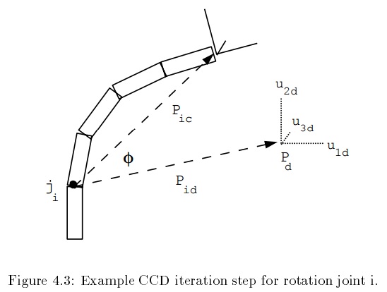
旋转型关节 Rotation Joint

图4.3演示了迭代过程中旋转型节点i的情况. 向量Pic是从节点位置Ji指向效应器位置的向量, Pid是从Ji指向期望的末端器位置的向量. 我们可以绕着世界空间的关节轴 axisi, 自由旋转向量Pic, 角度为Φ. 旋转后的向量为

P'ic(Φ) = Raxisi(Φ)Pic

随着Φ的改变, P'ic(Φ)划出一个以Ji为中心的圆圈. 圆上距离目标点Pd最近的点是圆与向量Pid的交点, 所以我们最好的做法是只偏移变量Ji偏移, 把P'ic(Φ)向Pid对齐. 这意味着我们需要找到一个Φ值, 使以下表达式的值最大

g1(Φ) = Pid·P'ic(Φ)　　(4.16)

用同样的方法 , 可以通过使下面的表达式最大化, 而朝向误差得到最佳矫正

g2(Φ) =  ∑j=13 ujd·u'jc(Φ)　　(4.17)

合并(4.16)和(4.17)这两个表达式, 得到节点i的一个聚合对象函数, 需要将它最大化,

g(Φ) = wpg1(Φ) + wog2(Φ)　　(4.18)

这里wp和wo是任意的位置和朝向加权因子, 他们的引入与雅可比转置法中, 为得到矩阵K而引入的因子类似. 为这两个因子设置的特殊值建议如下[WC91]

wo = 1

wp = α(1+ρ)

其中, α是一个缩放参数, 与世界缩放W按比例求反

α = k / W

这是为了这个算法的行为与缩放无关.因子ρ是一个任意的权重值, 与操纵器的配置相关. 虽然没有特别的原因, Wang[WC91]建议其取值为

ρ = min ( ||Pid||, ||Pic|| ) / max( ||Pid||, ||Pic|| )

这个值在实际使用中结果还算可以.

通过一些代数的计算, 在关节i处需要最大化的目标函数(4.18)可以简化为

g(Φ) = k1(1-cosΦ) + k2cosΦ + k3sinΦ　　(4.19)

 其中常量k1, k2, k3 的值分别为:

k1 = wp(Pid·axisi)(Pic·axisi) + wo∑j=13(ujd·axisi)(ujc·axisi)　　(4.20)

k2 = wp(Pid·Pic) wo∑j=13(ujd·ujc)　　　　　　　    　　　　　　　(4.21)

k3 = axisi·[wp(Pic x Pid) + wo∑j=13(ujc x ujd)]　　  　　　　　　(4.22)

根据初等微积分, 我们知道目标函数(4.19)在-π≤Φ≤-π的区间时, 在其一阶导数为0, 二阶导数为负数时, 可以达到最大值. 第一个条件

(k1 - k2)sinΦ + k3cosΦ = 0

意味着

Φ = tan-1(k3/(k2-k1))　　(4.23)

这样可以确定候选值Φc的取值范围是-π/2